After producing small area estimates using model based methods, their properties must be evaluated. This page discusses ways to evaluate the point estimates in terms of precision, accuracy and reliability and how to compare model based estimates with direct estimates.

Model-based or design-based simulation studies can be conducted to evaluate the method that was used to produce small area estimates. For a discussion on model and design based simulations, for method evaluation see Tzavidis et al. (2018).

Precision, accuracy and reliability

The precision of an estimator is usually evaluated by its variance. The bias on the other hand measures the accuracy of an estimator. A combined measure of precision and accuracy (variance and bias) is the mean squared error (MSE). A smaller MSE indicates that an estimate is more precise and/or accurate than a comparable estimate with a larger MSE. Every produced small area estimate should be accompanied with its MSE estimate. The MSE is defined by the expectation of the squared difference of the point estimate (mathjax-inline(\hat{\theta}_{i})mathjax-inline) and the true value (mathjax-inline(\theta_{i})mathjax-inline), at domain level (mathjax-inline(i)mathjax-inline) as follows

Since the true value is unknown, the MSE needs to be estimated. To estimate the MSE for model-based small area estimates, there exist different estimation methods:

  • analytical,
  • jackknife methods,
  • bootstrap methods.

For direct estimates, the MSE equals its variance because direct estimates are assumed to be unbiased. Estimates for the MSE are commonly returned by software packages. For methodological derivations and the estimated components of the MSE, please refer to the standard SAE literature.

In order to have comparable evaluation criteria independent of the scale of the indicator, the coefficient of variation (CV) is often used to assess estimates' reliability. It is given by the ratio of the square root of the estimated MSE and the point estimate at domain

Often, the CV is expressed as a percentage by multiplying it by 100.  Among statistical offices, the definition of sufficient reliability differs. The Office for National Statistics in the UK uses a top CV of 20% to define reliable estimates. The CV should be used with caution for ratios since the it could be high simply due to the fact that the point estimate is close to 0.

Comparison with direct estimates

Another way to evaluate the quality of the small area estimates is by comparing them with their direct counterparts. For areas with observations in the survey, the point estimate, the MSE and the CV can be compared. Especially for areas with many observations, the direct and small area estimates are expected to be very close to each other. The MSE of the model-based small area estimates is expected to be considerably lower than the MSE of the direct estimates because the model-based estimates borrow strength from similar areas.

In the practical exercise section different plots are presented that allow the practitioner to visually evaluate the small area model-based estimates in comparison to the direct estimates. 

SAEval - R package

The R package SAEval provides some methods proposed in Brown et al. (2001) to evaluate small area estimation, particularly by comparing direct and small area estimates.

Benchmarking

Model-based small area estimates can differ substantially from their direct counterparts. This is especially true for areas with very small sample size. Thus, totalling the disaggregated small area estimates to a higher aggregation level likely leads to differences between the higher-level direct estimates and the aggregated small area estimates (from the lower levels). The differences can be even more severe if the model is wrongly specified. Consistent estimates are, however, essential to convince policy makers from the correctness and usefulness of lower-level estimates. For indicators such as the mean, totals or proportions, a solution to this issue can be benchmarking. The goal of benchmarking is to adjust the produced model-based estimates in order to achieve coherence between the aggregated model-based estimates and the higher-level direct estimates. A very simple but popular benchmarking approach is the ratio adjustment approach. As described in Rao and Molina (2015), it is used to ensure that the benchmarked small area estimates    add up to a reliable direct estimate  with  , where (mathjax-inline(N_{i})mathjax-inline)  and (mathjax-inline(N)mathjax-inline)  are  respectively the domain and population sizes,and The adjusted model based estimate of area  is given by multiplying each small area estimate  by a common adjustment factor,

While the ratio benchmarking is easy to estimate, it has the downsides that each model based estimator is adjusted by the same adjustment factor not taking into account the precision of the model-based estimates. 

A benchmarking approach that can take the precision into account has been developed for area-level models by Datta et al. 2011. In this Bayesian approach, the benchmarked area-level estimator for domain is given by

where  is equal to the population share of each area. Depending on the weight , the formula allows for three different benchmarking options. 1) The weights used in the benchmarking, i.e.,   ; 2) Setting the weights  creates a ratio adjusted benchmarked estimator that takes into account the size of the point estimate; 3) In the last option , with (mathjax-inline(\bar{\hat{\theta}}_{\xi}^{EBLUP}= \sum_{i}^{D}\xi_{i}\hat{\theta}_{i}^{EBLUP})mathjax-inline), the benchmarking takes into account the precision. A detailed explanation of all three options is given in Datta et al. (2011).

There are also various other benchmarking methods for unit and area-level models, ranging from simple adjustment approaches, such as difference benchmarking to two-stage benchmarking and self-benchmarking (Rao and Molina 2015).


Practical exercise

The practical exercise in these guidelines will perform the analysis of three indicators for the SDGs 1, 7 and 8 with different input factors and estimation approaches. In this part, the evaluation and benchmarking of the produced estimators is described. The examples are chosen such that the application can be transferred to a wide range of SDG indicators.

1.1.1/1.2.1 Proportion of the population living below the international/national poverty line


Goal: For the proper planning of social support schemes, it could be of interest to target where the population below the national poverty line lives.

Indicator of interest: The proportion of the population living below the national poverty line. The proportion describes the fraction of the population with the characteristic of having, e.g., an income, below the poverty line and has a value between 0 and 1.

Disaggregation dimension: Required disaggregation dimensions for the indicator 1.2.1 are sex and age. However, the example only follows a spatial disaggregation by the second administrative level due to the common application of poverty mapping. The number of categories (domains) is 433 in the example.

Information about the household income is available in the survey syntheticSurvey1. The survey also contains variables that potentially explain the household income. Furthermore, a second data source, here the census (syntheticCensus), is available that does not contain the household income but the same explanatory variables as the survey. In both data sources, the domains defined by the second administrative level can be identified.

Load data sets
# Set working directory
setwd("Add path")


# Import sample and census at household level
survey <- read.csv("syntheticSurvey1.csv")
# The census csv was too large for the upload, thus it is available as RData file
load("syntheticCensus.RData")

# Overview of the variables
head(survey)
head(census)
First lines of data sets
> head(survey)
   eqIncome age sex yrschool              classwkd   geolev2 geolev1 electric urban
1 11997.722  30   1        5    wage/salary worker 170020016  170054      yes urban
2 24079.950  54   1        5    wage/salary worker 170070002  170013      yes urban
3 11737.735  51   1        3 niu (not in universe) 170073006  170073      yes urban
4 18713.431  25   1       13    wage/salary worker 170005049  170005      yes urban
5  9296.933  50   1       17    wage/salary worker 170063001  170066      yes urban
6 23142.577  59   0        0 niu (not in universe) 170005024  170005      yes urban


> head(census)
  age sex yrschool               classwkd   geolev2 geolev1
1  56   1       17 working on own account 170005001  170005
2  45   1       17     wage/salary worker 170005001  170005
3  47   1        5     wage/salary worker 170005001  170005
4  69   1       17  niu (not in universe) 170005001  170005
5  29   0        9        unknown/missing 170005001  170005
6  45   1       17     wage/salary worker 170005001  170005

The indicator of interest is a proportion (Mean or total? → No). Note that, technically, a proportion is the mean of a binary variable. This indicator, however, is calculated as a ratio since the number of households is also estimated based on survey data. The flowchart represents model choices related to linear and non-linear indicators (see SAE approaches).

The sample only has information of 152 of the 433 administrative regions, leaving 281 areas unsampled. The sample size in the administrative regions varies between 31 and 1024. Thus, there are regions with small sample sizes and unsampled regions (Small domains? → Yes). The available data is a household survey with the variable of interest and also a second data source at the unit-level, the census, is available (Unit-level data? → Yes).

This leads to SAE method group U2 in the figure above which means that a suitable approach for this example would be the ELL and the EBP. In the example, the EBP is used.

To estimate the regional distribution of the proportion of the population living below a poverty line, the specification based on the input factors leads to the EBP. To implement the analysis, a software package needs to be chosen. For this example, the R packages emdi and maptools are used. Please note that the proportion of the population living below a poverty line is defined as the head count ratio (HCR) in the package emdi. Thus, the proportion will be named as HCR in the following.

Load R packages
# Load packages
library(emdi)
library(maptools)

The EBP approach is based on a linear mixed regression model that links the variable of interest, the equivalized income, with covariates and categorical predictors, e.g., age and working class. To use the categorical variables in a  statistical model, they must be converted to factor variables in R. This lets the software know that it deals with categorical variables instead of numerical variables. 

Data preparation
# Data preparation -------------------------------------------------------------

# Convert categorical variables to factor variables
census$classwkd <- factor(census$classwkd)
census$sex <- factor(census$sex, levels = c(0,1), labels = c("m","f"))

survey$classwkd <- factor(survey$classwkd)
survey$urban <- factor(survey$urban)
survey$electric <- factor(survey$electric)
survey$sex <- factor(survey$sex, levels = c(0,1), labels = c("m","f")

The aim of the next step is to fit a suitable model. In the example, two different models are being compared. The first model (povEBP_reduced) uses "age", "sex" and "yrschool" as independent variables, whereas the second model additionally uses the variable "classwkd" as independent variable. It is expected, based on theoretical knowledge, that these covariates are associated with the equivalized household income. The default option for the poverty line in package emdi is 60% of the median of the dependent variable which is a common definition in the European Union. However, adding an argument for the threshold allows to use any required poverty line.

Model building
# Model building ---------------------------------------------------------------

# Linear mixed model without transformation
povEBP_reduced <- ebp(fixed = eqIncome ~ age + sex + yrschool, 
              pop_data = census, pop_domains = "geolev2", smp_data = survey, 
              smp_domains = "geolev2", na.rm = TRUE,  transformation = 'no', L = 1)

povEBP_full <- ebp(fixed = eqIncome ~ age + sex + yrschool + classwkd, 
              pop_data = census, pop_domains = "geolev2", smp_data = survey, 
              smp_domains = "geolev2", na.rm = TRUE,  transformation = 'no', L = 1)

# Check ICC and R2
summary(povEBP_reduced)
summary(povEBP_full)

# Check coefficients
summary(povEBP_full$model)

With the help of the summary function, sample sizes in the sample and the census are displayed, as well as some model diagnostics, e.g., the (mathjax-inline(R^2)mathjax-inline) and the ICC. While there are multiple methods and criteria that can be used to compare different models, the (mathjax-inline(R^2)mathjax-inline)  is used for this example. Based on the (mathjax-inline(R^2)mathjax-inline), the comparison shows that both models almost have an identical model goodness of fit. Because of the slight advantage of the full model over the reduced model it will be used going forward. The ICC indicates that there is unexplained heterogeneity between areas and the use of a random effects model is suitable.

Summary output
> summary(povEBP_reduced)
Empirical Best Prediction

Call:
 ebp(fixed = eqIncome ~ age + sex + yrschool, pop_data = census, 
    pop_domains = "geolev2", smp_data = survey, smp_domains = "geolev2", 
    L = 1, transformation = "no", na.rm = TRUE)

Out-of-sample domains:  281 
In-sample domains:  152 

Sample sizes:
Units in sample:  9155 
Units in population:  1007572 
                   Min. 1st Qu. Median       Mean 3rd Qu.  Max.
Sample_domains       31      35     41   60.23026   50.25  1024
Population_domains  521    1302   1651 2326.95612 2337.00 70499

Explanatory measures:
 Marginal_R2 Conditional_R2
   0.3880963      0.4395183

Residual diagnostics:
               Skewness Kurtosis Shapiro_W Shapiro_p
Error         1.1929905 5.365922        NA        NA
Random_effect 0.0382906 2.768383 0.9928648 0.6540751

ICC:  0.08403619 

Transformation: No transformation 

> summary(povEBP_full)
Empirical Best Prediction

Call:
 ebp(fixed = eqIncome ~ age + sex + yrschool + classwkd, pop_data = census, 
    pop_domains = "geolev2", smp_data = survey, smp_domains = "geolev2", 
    L = 1, transformation = "no", na.rm = TRUE)

Out-of-sample domains:  281 
In-sample domains:  152 

Sample sizes:
Units in sample:  9155 
Units in population:  1007572 
                   Min. 1st Qu. Median       Mean 3rd Qu.  Max.
Sample_domains       31      35     41   60.23026   50.25  1024
Population_domains  521    1302   1651 2326.95612 2337.00 70499

Explanatory measures:
 Marginal_R2 Conditional_R2
   0.3892696      0.4407805

Residual diagnostics:
                Skewness Kurtosis Shapiro_W Shapiro_p
Error         1.18494095 5.355828        NA        NA
Random_effect 0.03667253 2.778514  0.992828 0.6497688

ICC:  0.08434322 

Transformation: No transformation 

After an appropriate model was chosen the model assumptions must be checked. As before the output of the summary function provides information about the residuals. When looking at the skewness and kurtosis, it is obvious that the normality assumption of the unit-level (Error) is not fulfilled in this example. The skewness of a normal distribution is 0 and its kurtosis is 3. The normality assumption can also be checked with statistical tests like the Shapiro-Wilk test. For the random effects, the test suggests that the hypothesis of normality is not rejected. However, the results are not returned for the unit-level error terms since the corresponding function in R is only defined for sample sizes between 3 and 5.000. If the test of the unit-level errors is of interest, another test like the Kolmogorov-Smirnov could be chosen.

Another option to check the normality is to use the plot function on the model object that returns different plots, e.g., a QQ-plot of the unit- and area-level residuals.

Model assumptions
# Model assumptions ------------------------------------------------------------

# Check skewness, kurtosis, shapiro_w and shapiro_p test
summary(povEBP_full)

# Check plots
plot(povEBP_full)

The plot underlines what the skewness and kurtosis estimates also indicate, namely that the normality assumption for the unit-level error is not fulfilled.


To stay within the same model class and to meet the normality assumption of the EBP method, the log and the data driven Box-Cox transformations are applied to the dependent variable of the model. As before, the summary and the plot functions are used to get information about the distribution of the residuals.

Violated model assumptions
# Violated model assumptions ---------------------------------------------------

# Linear mixed model with Log transformation
povEBPLog <- ebp(fixed = eqIncome ~ age + sex + yrschool + classwkd, 
                   pop_data = census, pop_domains = "geolev2", smp_data = survey, 
                   smp_domains = "geolev2", na.rm = TRUE, transformation = 'log', L = 1)


# Linear mixed model with Box Cox transformation
povEBPBoxCox <- ebp(fixed = eqIncome ~ age + sex + yrschool + classwkd, 
                   pop_data = census, pop_domains = "geolev2", smp_data = survey, 
                   smp_domains = "geolev2", na.rm = TRUE, transformation = 'box.cox', L = 1)


# Compare skewness, kurtosis, shapiro_w and shapiro_p test
summary(povEBP_full)
summary(povEBPLog)
summary(povEBPBoxCox)

# Compare plots
plot(povEBP_full)
plot(povEBPLog)
plot(povEBPBoxCox)

The estimated skewness and kurtosis of the residuals obtained from the newly fitted models (with log and Box-Cox transformations) indicate that the normality assumption of the EBP method might not be violated anymore. For both models, the skewness of the residuals is close to 0 and the kurtosis is close to 3 (as expected for the normal distribution).

Output summary
> summary(povEBPLog)
Empirical Best Prediction

Call:
 ebp(fixed = eqIncome ~ age + sex + yrschool + classwkd, pop_data = census, 
    pop_domains = "geolev2", smp_data = survey, smp_domains = "geolev2", 
    L = 1, transformation = "log", na.rm = TRUE)

Out-of-sample domains:  281 
In-sample domains:  152 

Sample sizes:
Units in sample:  9155 
Units in population:  1007572 
                   Min. 1st Qu. Median       Mean 3rd Qu.  Max.
Sample_domains       31      35     41   60.23026   50.25  1024
Population_domains  521    1302   1651 2326.95612 2337.00 70499

Explanatory measures:
 Marginal_R2 Conditional_R2
   0.3895767      0.4776992

Residual diagnostics:
                 Skewness Kurtosis Shapiro_W Shapiro_p
Error          0.07490357 2.730150        NA        NA
Random_effect -0.28543231 3.246924 0.9921632 0.5728253

ICC:  0.1443628 

Transformation:
 Transformation Shift_parameter
            log               0

> summary(povEBPBoxCox)
Empirical Best Prediction

Call:
 ebp(fixed = eqIncome ~ age + sex + yrschool + classwkd, pop_data = census, 
    pop_domains = "geolev2", smp_data = survey, smp_domains = "geolev2", 
    L = 1, transformation = "box.cox", na.rm = TRUE)

Out-of-sample domains:  281 
In-sample domains:  152 

Sample sizes:
Units in sample:  9155 
Units in population:  1007572 
                   Min. 1st Qu. Median       Mean 3rd Qu.  Max.
Sample_domains       31      35     41   60.23026   50.25  1024
Population_domains  521    1302   1651 2326.95612 2337.00 70499

Explanatory measures:
 Marginal_R2 Conditional_R2
   0.3774885      0.4738446

Residual diagnostics:
                Skewness Kurtosis Shapiro_W Shapiro_p
Error         -0.1368913 2.888930        NA        NA
Random_effect -0.3890020 3.410824  0.988862 0.2696318

ICC:  0.1547861 

Transformation:
 Transformation Method Optimal_lambda Shift_parameter
        box.cox   reml     -0.2009575               0

Checking the QQ-plot of the newly fitted models' residuals confirms the prior findings. The next plot shows the results from the log model.

It is now up to the practitioner to decide if the model with either the log or the Box-Cox transformation should be used for producing the final estimates of the HCR, because both seem to fulfill the model assumptions quite well. In the next step, the final model (with log transformation) is fitted. The parameter L controls the number of Monte Carlo repetitions used in the EBP method. In the example, L is set to 100. Molina and Rao (2010) state that L=50 gives fairly accurate results but for practical applications they propose values larger than 200.

Fit final model
# Fit final model --------------------------------------------------------------

povEBP_final <- ebp(fixed = eqIncome ~ age + sex + yrschool + classwkd, 
                    pop_data = census, pop_domains = "geolev2", smp_data = survey, 
                    smp_domains = "geolev2", na.rm = TRUE, transformation = 'log', L = 100)


# Results per area -------------------------------------------------------------

# Table
estimators(povEBP_final, indicator = 'Head_Count', MSE = FALSE, CV = FALSE)

# Map
# Import shape file
geo2Shape <- readShapePoly("Add shapefile", delete_null_obj=TRUE)
map_plot(object = povEBP_final, MSE = FALSE, CV = FALSE, map_obj = geo2Shape,
         indicator = "Head_Count", map_dom_id = "GEOLEVEL2")

The estimated HCR per area can be printed in a table and plotted on a map. For the latter, a shape file needs to be available that contains the same regions for which the indicator is estimated for. Unfortunately, the shape file used in the example is too large to upload it such that it is not available for the user.

In the next figure, the produced map is plotted. Plotting the spatial distribution of the HCR enables policy makers to target political actions. 

Evaluation & Benchmarking

To evaluate the domain indicators, the model is fitted and the MSE and the CV are estimated. The estimation of the MSE and CV is triggered by setting the parameter MSE to "TRUE". In emdi, the MSE and CV are estimated using bootstrap methods. The parameter B controls the number of bootstrap iterations. It is advisable to set B to a minimum value of 100 in order to obtain reliable MSE estimates.

Precision, accuracy and reliability
# Precision, accuracy and reliability ------------------------------------------

# Fit model and bootstrap the MSE
povEBP_final <- ebp(fixed = eqIncome ~ age + sex + yrschool + classwkd, 
                    pop_data = census, pop_domains = "geolev2", smp_data = survey, 
                    smp_domains = "geolev2", na.rm = TRUE, transformation = 'log',
                    L = 100, MSE = TRUE, B = 100)

# Print disaggregated indicators with MSE and CV
head(estimators(povEBP_final, indicator = 'Head_Count', MSE = TRUE, CV = TRUE))

# Plot disaggregated CV
map_plot(object = povEBP_final, MSE = FALSE, CV = TRUE, map_obj = geo2Shape,
         indicator = "Head_Count", map_dom_id = "GEOLEVEL2")

The estimated regional indicators (the HCR in this example) with its MSE and CV can be obtained in the form of a table.

MSE and CV per area
> head(estimators(povEBP_final, indicator = 'Head_Count', MSE = TRUE, CV = TRUE))
     Domain Head_Count Head_Count_MSE Head_Count_CV
1 170005001 0.07658444   8.710772e-05    0.12186747
2 170005002 0.21080510   3.089281e-04    0.08337725
3 170005003 0.14358329   4.427159e-03    0.46340280
4 170005004 0.13571429   4.966465e-03    0.51927584
5 170005005 0.15856915   4.544493e-03    0.42513223
6 170005006 0.05288569   1.137584e-03    0.63775437

Additionally, the MSE and the CV can be plotted using the function map_plot. The results show that for some areas the estimated CV is considerably higher than 20% (threshold that is often used to argue that an estimator is reliable). This is a phenomenon often observed when working with ratio indicators. In the formula for the CV (given above), it is divided by the estimator (the estimated HCR). Hence, when the HCR takes on small values, the CV easily gets large.

To assess if the model-based HCR estimates are more reliable than the direct estimates various comparisons can be made. For sampled domains, the direct estimates and their CVs can be compared to the model-based estimates. Therefore, the direct estimates together with their variance are estimated. Afterwards, the CVs of the direct estimates are compared to the CVs of the model-based estimates.

Comparison with direct estimates
# Comparison with direct estimates ---------------------------------------------

# Estimate direct estimators for sampled domains
povDirect <- direct(y = "eqIncome", smp_data = survey,
                    smp_domains = "geolev2",var = TRUE, na.rm = TRUE, B = 100)

# Compare the CV between direct and model based estimates
compare_plot(povEBP_final, povDirect, indicator = 'Head_Count', MSE = FALSE, 
             CV = TRUE

The first plot shows a boxplot of the CVs of the HCR over the sampled areas for the model-based and direct estimates. The plot clearly indicates that the model based estimates are considerably more reliable than the direct estimates. Most of the model-based estimates have a CV of under 25%. The second plot presents the estimated CVs ordered by sample size (from large to small sample size). As expected, for large areas the estimated CV is comparable. With decreasing sample size the advantage of the model based method, in terms of lower CVs, is visible.


Additionally, the model-based estimated HCR can be compared to its direct counterpart. As expected, they are not identical but there is a strong linear relationship between them.

Before communicating the estimated indicators to policy makers, it can be desirable to benchmark the small area estimates to a direct national estimate. For estimating the direct national estimate, the whole sample is used. Afterwards, the popular but simple ratio adjustment method is applied to each model-based HCR estimate. 

Benchmarking
# Benchmarking -----------------------------------------------------------------

# Estimate national direct estimate using sample data
survey$national <- 1
direct_national <- direct(y = "eqIncome", smp_data = survey,
                          smp_domains = "national",var = FALSE, na.rm = TRUE)
hcr_national <- direct_national$ind$Head_Count

# Model based estimates
hcr_domain_model <- povEBP_final$ind$Head_Count

# Sample size per domain as proportion
domain_sample_size_proportion <- unname(
  table(povEBP_final$framework$pop_domains_vec))/
  sum(unname(table(povEBP_final$framework$pop_domains_vec)))

# Benchmarked model based estimates
hcr_domain_model_bench <- hcr_domain_model * (
  hcr_national/sum(domain_sample_size_proportion*hcr_domain_model))

df_benchmarked <- data.frame(hcr_domain_model, hcr_domain_model_bench)
colnames(df_benchmarked) <- c("Model based HCR", "Benchmarked model based HCR")

# Print results
head(df_benchmarked)

The results show that the benchmarked model based HCR estimates are all shrunk by the same factor of 0.88.

Benchmarked estimators
> head(df_benchmarked)
  Model based HCR Benchmarked model based HCR
1      0.07658444                  0.06754125
2      0.21080510                  0.18591299
3      0.14358329                  0.12662880
4      0.13571429                  0.11968898
5      0.15856915                  0.13984511
6      0.05288569                  0.04664089
7.1.1 Proportion of population with access to electricity

R Code

Goal: In order to have an idea if home schooling can work in rural and urban areas, it can be of interest to have information about the access to electricity which is a base requirement for digital education,

Indicator of interest: The proportion of population with access to electricity. The proportion describes the fraction of the population with the characteristic of having access to electricity and has a value between 0 and 1.

Disaggregation dimension: While the indicator does not have a required disaggregation dimension, the geographical location expressed in the two categories urban and rural is used in the example.

The variable describing households' access to electricity is contained in the household survey (syntheticSurvey1). Furthermore, a variable identifying rural and urban households is available.

Load data set
# Set working directory
setwd("Add path")

# Import sample and census at household level
survey <- read.csv("syntheticSurvey1.csv")

# First overview of data sets
head(survey)
First lines of data set
> head(survey)
   eqIncome age sex yrschool              classwkd   geolev2 geolev1 electric urban
1 11997.722  30   1        5    wage/salary worker 170020016  170054      yes urban
2 24079.950  54   1        5    wage/salary worker 170070002  170013      yes urban
3 11737.735  51   1        3 niu (not in universe) 170073006  170073      yes urban
4 18713.431  25   1       13    wage/salary worker 170005049  170005      yes urban
5  9296.933  50   1       17    wage/salary worker 170063001  170066      yes urban
6 23142.577  59   0        0 niu (not in universe) 170005024  170005      yes urban

The indicator of interest is a proportion (Mean or total? → No). This indicator is calculated as a ratio since the number of households is also estimated based on survey data.

The goal is to distinguish between urban and rural households. The sample size for the two categories is 3.125 for urban and 6.030 for rural (Small domains? → No). This leads to SAE method group D which suggests that direct estimation approaches can be sufficient. 

The sample sizes are large enough for the disaggregation requirement, even with the consideration of the information of interest if the household has access to electricity.

Check sample sizes in domains
# How small are the sample sizes for required disaggregation dimensions?
table(survey$urban)
table(survey$electric, survey$urban)
Sample sizes for disaggregation dimensions
> table(survey$urban)
rural urban 
 3125  6030

> table(survey$electric, survey$urban)
      rural urban
  no    679   117
  yes  2446  5913

To obtain estimates of the proportion of population with access to electricity, the specification based on the input factors leads to direct estimation. To implement the analysis, a software package needs to be chosen. For this example, the R package survey is used.

The survey data set is a sample from the census via simple random sampling. Thus, there is no sampling design that needs to be specified. However, in most real household surveys more complex survey designs are used. Thus, the R package survey is used for the following analysis since it is especially powerful for the analysis of survey data, also with complex survey designs. In a first step, the survey design needs to be specified with function svydesign.

Specify the sampling design
# The direct estimation is conducted with the survey package
library(survey)

# Specify the survey design (here the sampling was simple random sampling such 
# that no specific design needs to be specified but it is most likely the case
# in a real household survey)
samplingDesign <- svydesign(ids = ~1, data = survey)

The variable electric is a string variable with the options "yes" for electricity access and "no" if electricity access is not available. The function svymean automatically recognizes that the options are categories of a categorical variable and returns the proportions for both categories. With the help of function svyby, the proportions can be obtained for the geographic locations.

Get direct estimates
# The function notices that the string means two different categories 
svyby(~electric, ~urban, samplingDesign, svymean)

The output contains the point estimates as well as the corresponding standard errors. In urban regions, it is very unlikely not to have access to electricity but in rural area the proportion is at 22%.

Output
> svyby(~electric, ~urban, samplingDesign, svymean)
      urban electricno electricyes se.electricno se.electricyes
rural rural 0.21728000    0.782720   0.007377544    0.007377544
urban urban 0.01940299    0.980597   0.001776416    0.001776416

Evaluation & Benchmarking

To evaluate the domain indicators, the estimation is conducted and the MSE and the CV as measures for the uncertainty of the estimates are calculated. The estimation of the standard errors is automatically returned along with the point estimates. For the estimation of the CV, the function cv can be used. The CVs are far below the threshold of 20%. Thus, the direct estimation would be sufficient at this disaggregation dimension.

Precision, accuracy and reliability
cv(svyby(~electric, ~urban, samplingDesign, svymean))
Variance and CV estimates
> cv(svyby(~electric, ~urban, samplingDesign, svymean))
      se.electricno se.electricyes
rural    0.03395409    0.009425521
urban    0.09155374    0.001811566

Benchmarking

Direct estimates have the property to sum up to the population estimate such that benchmarking is not necessary.

8.5.2 Unemployment rate

R Code

Goal: Employment is often a key against hunger and extreme poverty. Thus, the identification of groups without employment could be of interest in order to counteract their unemployment with specialized programs.

Indicator of interest: The unemployment rate defined as the number of unemployed persons divided by the total number of working-age persons in the labour force. The unemployment rate is a proportion describing the fraction of the labor force with the characteristic to be unemployed and has a value between 0 and 1. In the example, the working age is defined between 15 and 74.

Disaggregation dimension: The required disaggregation dimensions are sex, age, geographic location (urban/rural), and disability status. The example will consider these dimensions and show some limitations and challenges.

Information about the employment status is available in the survey of the working population (syntheticSurvey2). The data further contains variables for the different disaggregation dimensions, The aggregated data sets contain variables that could help to explain the unemployment rate at different domain levels.

Load data sets
# Set working directory
setwd("Add path")

# Import sample and census at household level
survey2 <- read.csv("syntheticSurvey2.csv")
# Import aggregated data sets
auxiliaryAgeGeographic <- read.csv("auxiliaryAgeGeographic.csv")
auxiliarySexSpatial <- read.csv("auxiliarySexSpatial.csv")


# First overview of data sets
head(survey2)
head(auxiliaryAgeGeographic)
head(auxiliarySexSpatial)
First lines of data sets
> head(survey2)
  unemployed geolev1 urban age    sex         disabled ageGroup1 ageGroup2   weight
1          0  170005 urban  17   male no, not disabled     15-24     15-19 99.83459
2          0  170005 urban  58   male    yes, disabled     45-64     55-59 99.83459
3          0  170005 urban  15   male no, not disabled     15-24     15-19 99.83459
4          1  170005 urban  33 female no, not disabled     25-44     30-34 99.83459
5          0  170005 urban  34   male no, not disabled     25-44     30-34 99.83459
6          1  170005 urban  30   male no, not disabled     25-44     30-34 99.83459

> head(auxiliaryAgeGeographic)
       domain classwk_niu classwk_self_employed classwk_unknown classwk_unpaid_worker classwk_salary_worker
1 15-19.rural  0.04476600             0.1262039      0.02371693            0.09226769             0.7130454
2 20-24.rural  0.03706738             0.1535128      0.02428678            0.02421396             0.7609190
3 25-29.rural  0.02094564             0.1835557      0.02432163            0.01586351             0.7553135
4 30-34.rural  0.01368511             0.2085479      0.02479579            0.01252371             0.7404475
5 35-39.rural  0.01093352             0.2292661      0.02178753            0.01117207             0.7268408
6 40-44.rural  0.01009656             0.2524360      0.02259601            0.01181606             0.7030554
  edattain_less_than_primary_completed edattain_primary_completed edattain_secondary_completed edattain_university_completed edattain_unknown
1                            0.3369659                  0.5581732                   0.09767126                  0.0001130454      0.007076645
2                            0.3266517                  0.4485408                   0.20982395                  0.0083201340      0.006663390
3                            0.3924313                  0.4100554                   0.17023323                  0.0208367365      0.006443416
4                            0.4583640                  0.3925709                   0.11648794                  0.0261313925      0.006445743
5                            0.5042343                  0.3693344                   0.08955550                  0.0296199109      0.007255884
6                            0.5572726                  0.3349720                   0.07052158                  0.0296283233      0.007605485

> head(auxiliarySexSpatial)
         domain classwk_niu classwk_self_employed classwk_unknown classwk_unpaid_worker classwk_salary_worker
1 female.170005  0.01998601             0.1309242      0.05098013           0.009451625             0.7886580
2   male.170005  0.01475410             0.2249606      0.02876725           0.005483005             0.7260350
3 female.170008  0.06420981             0.1770292      0.03496872           0.014771271             0.7090210
4   male.170008  0.07113928             0.3236331      0.02970074           0.009375234             0.5661517
5 female.170011  0.01891617             0.1630182      0.02206017           0.006888095             0.7891173
6   male.170011  0.01502477             0.2279818      0.01806746           0.003034830             0.7358912
  edattain_less_than_primary_completed edattain_primary_completed edattain_secondary_completed edattain_university_completed edattain_unknown
1                            0.1566849                  0.2839548                    0.4182401                    0.13812005      0.003000158
2                            0.3805409                  0.3500880                    0.2126424                    0.05398722      0.002741502
3                            0.1140252                  0.2600799                    0.3934735                    0.23023589      0.002185545
4                            0.2128178                  0.3372084                    0.3350709                    0.11257781      0.002325058
5                            0.1033345                  0.3216923                    0.3652386                    0.20833877      0.001395883
6                            0.2118720                  0.3944650                    0.2628273                    0.12954635      0.001289410

The indicator of interest is a proportion (Mean or total? → No). This indicator is calculated as a ratio since the working-age population in the labor force is also estimated based on survey data.

The goal is to try different disaggregation dimensions. For the disaggregation dimensions sex, age group, geographic location (urban/rural), and disability status direct estimates are obtained assuming that the sample sizes are large enough (Small domains? → No). For a combination of the dimensions age group and geographic location, as well as sex and administrative region, area-level models are applied, assuming that the precision could be improved compared to the direct estimates (Small domains? → Yes) and considering that only aggregated auxiliary data is available (Unit-level data? → No).

The sample sizes are relatively large for all single disaggregation dimensions (except for unknown disability status). The cross-classification of disaggregation variables dimensions partly lead to smaller sample sizes.

Check sample sizes
# How small are the sample sizes for required disaggregation dimensions?
table(survey2$sex)
table(survey2$ageGroup1)
table(survey2$ageGroup2)
table(survey2$urban)
table(survey2$disabled)

table(survey2$sex, survey2$geolev1)
table(survey2$ageGroup2, survey2$urban)

table(survey2$unemployed, survey2$ageGroup2, survey2$urban)
Sample sizes for disaggregation dimensions
> table(survey2$sex)
female   male 
  5747  15813 

> table(survey2$ageGroup1)
15-24 25-44 45-64   65+ 
 4234 11131  5420   775 

> table(survey2$ageGroup2)
15-19 20-24 25-29 30-34 35-39 40-44 45-49 50-54 55-59 60-64   65+ 
 1544  2690  2908  2942  2742  2539  2076  1560  1097   687   775 

> table(survey2$urban)
rural urban 
 8806 12754 

> table(survey2$disabled)
no, not disabled          unknown    yes, disabled 
           20143               17             1400 

> table(survey2$ageGroup2, survey2$urban)       
        rural urban
  15-19   865   679
  20-24  1134  1556
  25-29  1095  1813
  30-34  1149  1793
  35-39   987  1755
  40-44   946  1593
  45-49   767  1309
  50-54   598   962
  55-59   487   610
  60-64   339   348
  65+     439   336

> table(survey2$sex, survey2$geolev1)        
         170005 170008 170011 170013 170015 170018 170019 170023 170027 170041 170044 170050 170052 170054 170066 170068 170073 170076 170081
  female    666    215   1004    325    387     83    318    141     68    131     86    123    302    351    399    288    217    443     47
  male     1872    508   1963   1332   1124    231    926    599    172    635    183    323    870   1142   1049    849    667    987    105
        
         170086 170088 170095
  female     62     16     75
  male      122     34    120

Considering the groups of employed and unemployed highlights a low number of unemployed population in some domains (exemplary for the combination of age groups and geographic location).

Sample sizes for disaggregation dimensions by category
> table(survey2$unemployed, survey2$ageGroup2, survey2$urban)
, ,  = rural
    15-19 20-24 25-29 30-34 35-39 40-44 45-49 50-54 55-59 60-64  65+
  0   815  1051  1049  1111   961   918   745   582   479   331  434
  1    50    83    46    38    26    28    22    16     8     8    5

, ,  = urban
    15-19 20-24 25-29 30-34 35-39 40-44 45-49 50-54 55-59 60-64  65+
  0   581  1365  1697  1681  1660  1524  1248   892   589   334  315
  1    98   191   116   112    95    69    61    70    21    14   21

The goal of the analysis is to obtain estimates of the unemployment rate for different disaggregation dimensions. The following descriptions will be focused on the combination of the dimensions age group and geographic location. 

To estimate the unemployment rate for the different disaggregation dimensions, the specification based on the input factors leads to direct estimation and an area-level model. To implement the analysis, a software package needs to be chosen. For this example, the R packages survey and emdi are used (for the data management, also package reshape2 is loaded).

The survey data set contains sampling weights to correct the differences in selection probabilities. One popular R package for the analysis of survey data, especially with complex survey designs, is the survey package. The survey design can be specified with function svydesign. In this example, the survey design is specified with the sampling weights.

Specify the sampling design
# For a first analysis, direct estimation is conducted with the survey package
library(survey)

# Specify the survey design
samplingDesign <- svydesign(ids = ~1, weights = ~weight, data = survey2)

The variable unemployment is 1, when the person is unemployed, and 0, when the person is employed. Thus, the unemployment rate can be directly estimated by taking the mean within the required disaggregation dimension. The function svyby enables the operation of function svymean for the estimation of the mean and its standard error by the required disaggregation dimension considering the sampling design.

Get direct estimates
# Unemployment rate by combination of age groups and geographic location 
svyby(~unemployed, ~ageGroup2 + urban, samplingDesign, svymean)

For the combination of age groups in five year intervals and the geographic location, it is apparent that the unemployment rate is especially high for the young urban population with 14% in the age group 15-19.

Output
> svyby(~unemployed, ~ageGroup2 + urban, samplingDesign, svymean)
            ageGroup2 urban unemployed          se
15-19.rural     15-19 rural 0.06056085 0.009828506
20-24.rural     20-24 rural 0.07150598 0.008691182
25-29.rural     25-29 rural 0.03741252 0.006284867
30-34.rural     30-34 rural 0.03192538 0.006060037
35-39.rural     35-39 rural 0.02243432 0.005381977
40-44.rural     40-44 rural 0.02927986 0.006382300
45-49.rural     45-49 rural 0.02200518 0.005277605
50-54.rural     50-54 rural 0.01985975 0.005739776
55-59.rural     55-59 rural 0.01898093 0.007267124
60-64.rural     60-64 rural 0.02538600 0.009504805
65+.rural         65+ rural 0.01107436 0.005740872
15-19.urban     15-19 urban 0.14233478 0.015490624
20-24.urban     20-24 urban 0.12001686 0.009406144
25-29.urban     25-29 urban 0.05580399 0.005981996
30-34.urban     30-34 urban 0.06480648 0.006693129
35-39.urban     35-39 urban 0.05163059 0.005949129
40-44.urban     40-44 urban 0.04330892 0.005920045
45-49.urban     45-49 urban 0.05145245 0.007122834
50-54.urban     50-54 urban 0.08046659 0.010350335
55-59.urban     55-59 urban 0.03489428 0.008645406
60-64.urban     60-64 urban 0.03867333 0.011588445
65+.urban         65+ urban 0.07394510 0.017770256

While the direct estimation does not require any model building or checking, it is the starting point for the area-level model. The first set of inputs required for a basic area-level model are the direct estimates and their sampling error variances. While the sampling error variance is assumed to be known, it usually needs to be estimated from unit-level data (see Estimation of the sampling error variance for more information). In this application, the indicator of interest is a proportion defined between 0 and 1. Thus, it is recommended to use either a different model specification for variables between 0 and 1 or to use the arcsin transformation. The latter option is chosen since it allows to stay within the same model class. To apply the transformed area-level model, an approximation for the sampling error variance is needed. Thus, the effective sample size needs to be calculated. The design effect can be estimated with the svymean function from the survey package. The effective sample size is estimated by the division of the sample size and the design effect (Casas-Cordero, Encina e Lahiri, 2016).

Data preparation for area-level model application
# Get the direct estimate and the design effect
directEstim <- svyby(~unemployed, ~ageGroup2 + urban, samplingDesign, svymean, deff = TRUE)
directEstim <- directEstim[, c('unemployed', 'se', 'DEff.unemployed')]
directEstim$domain <- row.names(directEstim)

# Calculate the sample size for the domains
library(reshape2)
sampleSize <- melt(table(survey2$ageGroup2, survey2$urban))
sampleSize$domain <- paste0(sampleSize$Var1, '.', sampleSize$Var2)

# Merge the direct estimate and the sample size
directEstim <- merge(directEstim, sampleSize[, c('domain', 'value')], by = 'domain')

# Calculate the effectice sample size
directEstim$effSampleSize <- directEstim$value/directEstim$DEff.unemployed

# Calculate the variance
directEstim$directVar <- directEstim$se^2

# Reduce to relevant variables
directEstim <- directEstim[, c('domain', 'unemployed', 'effSampleSize', 'directVar')]
Output
> directEstim
        domain unemployed effSampleSize    directVar
1  15-19.rural 0.06056085      577.7407 9.659952e-05
2  15-19.urban 0.14233478      500.7557 2.399594e-04
3  20-24.rural 0.07150598      861.5977 7.553665e-05
4  20-24.urban 0.12001686     1174.5608 8.847555e-05
5  25-29.rural 0.03741252      893.9596 3.949955e-05
6  25-29.urban 0.05580399     1448.8465 3.578428e-05
7  30-34.rural 0.03192538      824.8754 3.672405e-05
8  30-34.urban 0.06480648     1330.6919 4.479797e-05
9  35-39.rural 0.02243432      742.4734 2.896567e-05
10 35-39.urban 0.05163059     1360.5912 3.539214e-05
11 40-44.rural 0.02927986      684.2333 4.073376e-05
12 40-44.urban 0.04330892     1162.5466 3.504693e-05
13 45-49.rural 0.02200518      757.5538 2.785311e-05
14 45-49.urban 0.05145245      946.6877 5.073477e-05
15 50-54.rural 0.01985975      579.5396 3.294503e-05
16 50-54.urban 0.08046659      679.5051 1.071294e-04
17 55-59.rural 0.01898093      346.3156 5.281110e-05
18 55-59.urban 0.03489428      443.4726 7.474305e-05
19 60-64.rural 0.02538600      268.9703 9.034132e-05
20 60-64.urban 0.03867333      272.8263 1.342920e-04
21   65+.rural 0.01107436      326.1544 3.295761e-05
22   65+.urban 0.07394510      213.4372 3.157820e-04

The second set of inputs is the aggregated auxiliary information at the domain level. To use the package emdi for the analysis, the two data sets need to be combined into one. While the data preparation steps above can differ depending on the data set used, the data set that is given to the function fh in the package emdi needs to look like the combined data set below, containing the direct estimate, the sampling error variance (here estimated by the direct variance), the effective sample size (if the arcsin transformation is applied), and the auxiliary variables.

Combine data sets
# Combine the survey data with the additional data source
combined_data <- merge(directEstim, auxiliaryAgeGeographic, by = 'domain')
head(combined_data)
First lines of combined data set
> head(combined_data)
       domain unemployed effSampleSize    directVar classwk_niu classwk_self_employed classwk_unknown classwk_unpaid_worker
1 15-19.rural 0.06056085      577.7407 9.659952e-05  0.04476600            0.12620393      0.02371693           0.092267692
2 15-19.urban 0.14233478      500.7557 2.399594e-04  0.10781630            0.08427786      0.03029295           0.048356147
3 20-24.rural 0.07150598      861.5977 7.553665e-05  0.03706738            0.15351284      0.02428678           0.024213957
4 20-24.urban 0.12001686     1174.5608 8.847555e-05  0.06567831            0.10625758      0.02763255           0.008663353
5 25-29.rural 0.03741252      893.9596 3.949955e-05  0.02094564            0.18355568      0.02432163           0.015863508
6 25-29.urban 0.05580399     1448.8465 3.578428e-05  0.03302284            0.15582710      0.03055306           0.004865550
  classwk_salary_worker edattain_less_than_primary_completed edattain_primary_completed edattain_secondary_completed
1             0.7130454                           0.33696586                  0.5581732                   0.09767126
2             0.7292567                           0.14210055                  0.4969170                   0.35804017
3             0.7609190                           0.32665174                  0.4485408                   0.20982395
4             0.7917682                           0.08839411                  0.3060407                   0.53568936
5             0.7553135                           0.39243126                  0.4100554                   0.17023323
6             0.7757315                           0.10186204                  0.2872987                   0.44789884
  edattain_university_completed edattain_unknown
1                  0.0001130454      0.007076645
2                  0.0012025074      0.001739798
3                  0.0083201340      0.006663390
4                  0.0683943275      0.001481466
5                  0.0208367365      0.006443416
6                  0.1617471579      0.001193262

The aim of the next step is to fit a suitable model. The auxiliary data has information of working class and educational attainment. Both categorical predictors are potentially associated with employment status. Thus, two models are built and compared. For fitting the model, the R package emdi is used since it provides the option of using the arcsin transformation. The bias-corrected backtransformation is chosen (bc) instead of a naive backtransformation.

Model building
# Model building ---------------------------------------------------------------
# Load package emdi for model fitting
library(emdi)

# Model with educational attainment
unemplFH1 <- fh(fixed = unemployed ~ edattain_less_than_primary_completed + 
               edattain_primary_completed + edattain_secondary_completed +
               edattain_university_completed,
             vardir = "directVar", combined_data = combined_data, domains = "domain",
             method = 'ml', transformation = "arcsin", backtransformation = "bc",
             eff_smpsize = "effSampleSize")
summary(unemplFH1)

# Mode with working class
unemplFH2 <- fh(fixed = unemployed ~ classwk_unpaid_worker + classwk_salary_worker + 
               classwk_niu + classwk_self_employed, 
             vardir = "directVar", combined_data = combined_data, domains = "domain",
             method = 'ml', transformation = "arcsin", backtransformation = "bc", 
             eff_smpsize = "effSampleSize")
summary(unemplFH2)

With the help of the summary function, the practitioner gets information about the number of domains as well as some model diagnostics, e.g., the information criteria and the (mathjax-inline(R^2)mathjax-inline). While there are multiple methods and criteria that can be used to compare different models; in this example, the focus is on the information criteria and the adjusted (mathjax-inline(R^2)mathjax-inline). Since the information criteria AIC and BIC are smaller in unemplFH2 and the adjusted (mathjax-inline(R^2)mathjax-inline) is larger for this model, it will be used going forward. Please note that the estimation method for the parameters needs to be set to maximum likelihood if the information criteria will be used for the model selection.

Output summary
> summary(unemplFH1)
Call:
 fh(fixed = unemployed ~ edattain_less_than_primary_completed + 
    edattain_primary_completed + edattain_secondary_completed + 
    edattain_university_completed, vardir = "directVar", 
    combined_data = combined_data, domains = "domain", 
    method = "ml", transformation = "arcsin", backtransformation = "bc", 
    eff_smpsize = "effSampleSize")

Out-of-sample domains:  0 
In-sample domains:  22 

Variance and MSE estimation:
Variance estimation method:  ml 
Estimated variance component(s):  0.0006418727 
MSE method:  no mse estimated 

Coefficients:
                                     coefficients std.error   t.value     p.value
(Intercept)                             -15.95450  6.017710 -2.651257 0.008019284
edattain_less_than_primary_completed     16.24525  6.093368  2.666054 0.007674728
edattain_primary_completed               16.30899  6.033234  2.703192 0.006867715
edattain_secondary_completed             16.41763  6.030143  2.722594 0.006477162
edattain_university_completed            15.64274  5.932548  2.636765 0.008370069

Explanatory measures:
  loglike      AIC       BIC        R2     AdjR2
1 43.8617 -75.7234 -69.17714 0.7071698 0.7725552

Residual diagnostics:
                        Skewness Kurtosis Shapiro_W Shapiro_p
Standardized_Residuals 0.8565795 3.109786 0.9275953 0.1093302
Random_effects         0.7580138 3.594312 0.9276477 0.1096054

Transformation:
 Transformation Back_transformation
         arcsin                  bc
> summary(unemplFH2)
Call:
 fh(fixed = unemployed ~ classwk_unpaid_worker + classwk_salary_worker + 
    classwk_niu + classwk_self_employed, vardir = "directVar", 
    combined_data = combined_data, domains = "domain", 
    method = "ml", transformation = "arcsin", backtransformation = "bc", 
    eff_smpsize = "effSampleSize")

Out-of-sample domains:  0 
In-sample domains:  22 

Variance and MSE estimation:
Variance estimation method:  ml 
Estimated variance component(s):  0.000322217 
MSE method:  no mse estimated 

Coefficients:
                      coefficients std.error   t.value      p.value
(Intercept)               5.220890  1.241659  4.204771 2.613461e-05
classwk_unpaid_worker    -5.487824  1.180430 -4.649004 3.335425e-06
classwk_salary_worker    -5.126887  1.258385 -4.074181 4.617651e-05
classwk_niu              -3.299256  1.548756 -2.130262 3.314998e-02
classwk_self_employed    -5.349499  1.321804 -4.047119 5.185180e-05

Explanatory measures:
   loglike       AIC      BIC        R2     AdjR2
1 48.56608 -85.13215 -78.5859 0.8139054 0.8835492

Residual diagnostics:
                        Skewness Kurtosis Shapiro_W Shapiro_p
Standardized_Residuals 0.7114812 3.428400 0.9479491 0.2874469
Random_effects         0.5690609 3.584361 0.9606795 0.5031370

Transformation:
 Transformation Back_transformation
         arcsin                  bc

After an appropriate model is chosen the model assumptions must be checked. As before the summary function provides information about the residuals and the random effects. When looking at the skewness and kurtosis, it seems that the kurtosis estimates for the distribution of the residuals and random effects are compatible with a a normal distribution but that the data is slightly skewed. The skewness of a normal distribution is 0 and its kurtosis is 3. The Shapiro-Wilk test that tests the hypothesis whether the data follows normal distribution does not reject the normality of the residuals and random effects. Another option to check the normality assumption can be various plots, e.g., a QQ plot that can be produced with the plot function.

Model assumptions
# Model assumptions ------------------------------------------------------------

# Check skewness, kurtosis, shapiro_w and shapiro_p test
summary(unemplFH2)

# Check diagnostic plots
plot(unemplFH2)

The QQ plots show a difficulty of this application. The area-level model is conducted with only 22 domains in this example. With a small number of domains, it is more likely that the Shapiro-Wilk test will not reject the normality (the null hypotheses). The QQ plots may help to confirm or to reject the normality assumption. However, it is also up for interpretation. For the following, the model unemplFH2 is used as a final model assuming no violation of the model assumptions.


After checking the model, the final model can be fitted. The estimators function returns a table that allows a fast comparison of the model-based estimates with the direct estimates. For the final model, the default estimation which is restricted maximum likelihood is used in this example.

Fit final model
# Fit final model --------------------------------------------------------------

unemplFH2 <- fh(fixed = unemployed ~ classwk_unpaid_worker + classwk_salary_worker + 
                  classwk_niu + classwk_self_employed, 
                vardir = "directVar", combined_data = combined_data, domains = "domain",
                transformation = "arcsin", backtransformation = "bc", 
                eff_smpsize = "effSampleSize")

estimators(unemplFH2)

The returned table of point estimates shows that the estimates are quite similar for the domains.

Point estimates
> estimators(unemplFH2)
Indicator/s: All indicators
        Domain     Direct         FH
1  15-19.rural 0.06056085 0.05811014
2  15-19.urban 0.14233478 0.15020506
3  20-24.rural 0.07150598 0.06667850
4  20-24.urban 0.12001686 0.11536616
5  25-29.rural 0.03741252 0.03974987
6  25-29.urban 0.05580399 0.06016464
7  30-34.rural 0.03192538 0.03420204
8  30-34.urban 0.06480648 0.06473852
9  35-39.rural 0.02243432 0.02509315
10 35-39.urban 0.05163059 0.05036153
11 40-44.rural 0.02927986 0.02892317
12 40-44.urban 0.04330892 0.04197867
13 45-49.rural 0.02200518 0.02476735
14 45-49.urban 0.05145245 0.04953178
15 50-54.rural 0.01985975 0.02062209
16 50-54.urban 0.08046659 0.06542743
17 55-59.rural 0.01898093 0.02031048
18 55-59.urban 0.03489428 0.04331501
19 60-64.rural 0.02538600 0.01816915
20 60-64.urban 0.03867333 0.04617507
21   65+.rural 0.01107436 0.01606912
22   65+.urban 0.07394510 0.06862117

Evaluation & Benchmarking

To evaluate the domain indicators, the model is fitted and the MSE and the CV as measure for the uncertainty of the estimates are calculated. The estimation of the MSE and CV is triggered by setting the parameter MSE to "TRUE". For the transformed area-level model with bias-corrected backtransformation, a bootstrap MSE is provided. The parameter B controls the number of bootstrap iterations. It is advisable to set B to a minimum value of 100 to obtain reliable MSE estimates.

Precision, accuracy and reliability
# Evaluation -------------------------------------------------------------------

unemplFH2 <- fh(fixed = unemployed ~ classwk_unpaid_worker + classwk_salary_worker + 
                  classwk_niu + classwk_self_employed, 
                vardir = "directVar", combined_data = combined_data, domains = "domain",
                transformation = "arcsin", backtransformation = "bc", 
                eff_smpsize = "effSampleSize", MSE = TRUE, mse_type = 'boot', 
                B = 100)

estimators(unemplFH2, MSE = TRUE, CV = TRUE)
head(estimators(unemplFH2, MSE = TRUE, CV = TRUE))

The estimated regional indicators (the unemployment rate in this example) with its MSE and CV can be obtained in the form of a table. Generally, the CV should be used with caution when the indicator of interest is a ratio since point estimates close to zero can also be the reason for large CVs. In these cases, it is recommendable to focus on the MSE.

In this example, the CV of the model-based estimate (FH) is generally lower than for the direct estimate. However, there are also cases where the CV is slightly larger. One reason could be that the number of bootstrap iterations is too small.

MSE and CV per domain
> head(estimators(unemplFH2, MSE = TRUE, CV = TRUE))
       Domain     Direct   Direct_MSE  Direct_CV         FH       FH_MSE      FH_CV
1 15-19.rural 0.06056085 9.659952e-05 0.16229141 0.05811014 8.992932e-05 0.16319196
2 15-19.urban 0.14233478 2.399594e-04 0.10883232 0.15020506 2.052526e-04 0.09538053
3 20-24.rural 0.07150598 7.553665e-05 0.12154483 0.06667850 3.694515e-05 0.09115761
4 20-24.urban 0.12001686 8.847555e-05 0.07837353 0.11536616 4.120060e-05 0.05563823
5 25-29.rural 0.03741252 3.949955e-05 0.16798831 0.03974987 4.805691e-05 0.17439831
6 25-29.urban 0.05580399 3.578428e-05 0.10719657 0.06016464 4.202419e-05 0.10774778

The model-based estimates are commonly compared with the results of direct estimates. The function compare_plot in emdi provides some plots for this comparison. 

Comparison with direct estimation
# Comparison with direct estimates
compare_plot(unemplFH2, MSE = TRUE, CV = TRUE)

Comparing direct with model-based estimates helps to evaluate if the model-based estimates are more reliable than the direct estimates measured in terms of the MSE or the CV. The boxplots confirm that the model-based estimates have lower CVs overall. Approximately, 75% of the model-based domain estimates show a CV below 20%. It is also apparent that the increase in efficiency is not huge. Furthermore, the second plot (on the right) shows that there are also domains where the CV of the model-based estimates is slightly larger than those of corresponding direct estimates.

When comparing the direct and model-based point estimates, it can be seen that these do not differ strongly from each other.

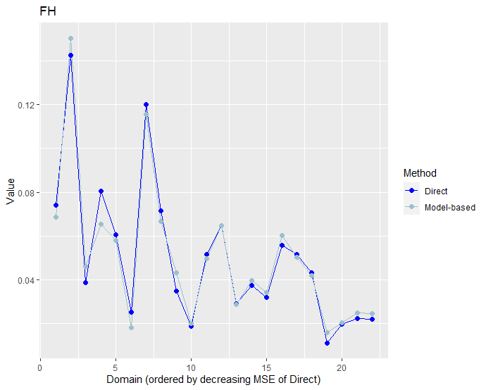
This could be due to a large weight on the direct estimator. For this, the estimated shrinkage factor can be checked. Furthermore, the Brown test can be conducted and the correlation between the direct estimates and the estimates of the regression-synthetic part can be calculated with the function compare. 

Comparison with direct estimation (continued)
# Summary of estimates shrinkage factor
summary(unemplFH2$model$gamma$Gamma)
# Brown test and correlation between direct estimates and regression-synthetic part
compare(unemplFH2)

The results show that the weight on the direct estimate ranges between 0.3 and 0.75 with a median of 0.6. Thus, the weight on the direct estimate is relatively high. Furthermore, the hypothesis that the model-based estimates differ from the direct estimates is not rejected and the correlation between the direct estimates and the regression-synthetic part is high with 0.93.

Comparison with direct estimation (continued)
> summary(unemplFH2$model$gamma$Gamma)
   Min. 1st Qu.  Median    Mean 3rd Qu.    Max. 
 0.3050  0.4845  0.5944  0.5680  0.6574  0.7487 
> compare(unemplFH2)
Brown test 

Null hypothesis: EBLUP estimates do not differ significantly from the 
      direct estimates 

  W.value Df   p.value
 4.547096 22 0.9999734

Correlation between synthetic part and direct estimator:  0.93 

Before communicating the estimated indicators to policy makers, it is common practice to to benchmark the small area estimates to a direct population estimate. For estimating the direct population estimate, the whole sample is used. In this example, the aggregation of the model-based domain estimates is about 5.5%, already quite close to the direct population estimate of 5.6%. This is due to the fact that the model-based domain estimates are close to the direct domain estimates. To ensure the direct population estimate, the benchmarking following Datta et al. (2011) (option 1) is used in this example. To conduct the benchmarking the population shares per domain are needed.

Download population shares

Benchmarking
# Benchmarking -----------------------------------------------------------------

# Calculate population direct estimate
svymean(~unemployed, samplingDesign)

# Load population shares
sharePopulationSize <- read.csv('sharePopulationSize.csv')

# To ensure the same ordering, the data sets are merged
share <- merge(unemplFH2$ind, sharePopulationSize, by.x = 'Domain', by.y = 'domain')

# The model-based estimate almost equals to the direct estimate
sum(share$ratio_n * unemplFH2$ind$FH)

# Benchmarking with raking 
unemplFH2_benchmarked <- benchmark(unemplFH2, benchmark = 0.056111,
                                   share = share$ratio_n)

# The benchmarked value equals the direct estimate
sum(share$ratio_n * unemplFH2_benchmarked$FH_Bench)

# Benchmarked point estimates
head(unemplFH2_benchmarked)

The benchmarking changes the estimates only slightly.

Benchmarked estimates
> head(unemplFH2_benchmarked)
       Domain     Direct         FH   FH_Bench Out
1 15-19.rural 0.06056085 0.05811014 0.05865782   0
2 15-19.urban 0.14233478 0.15020506 0.15075274   0
3 20-24.rural 0.07150598 0.06667850 0.06722618   0
4 20-24.urban 0.12001686 0.11536616 0.11591384   0
5 25-29.rural 0.03741252 0.03974987 0.04029754   0
6 25-29.urban 0.05580399 0.06016464 0.06071232   0

No interpretation of results

Please note that none of the results can be interpreted in any way. The data provided is solely used to explain the methods and how to conduct a study, and are not meant for a real analysis.

  • No labels